Here you will find out latest app notes.
Analog behavior modeling (ABM) allows the simulation of analog circuits using mathematical equations. This application note shows how the filter behavioral models are developed and implemented using the Laplace function of PSpice, Given the filter bandwidth and order, the models simulate lowpass, highpass, bandpass, and band-reject filters. For ease of use, the models are developed as parameterized sub-circuits. Simulation examples are included to demonstrate the use of these models.
By Bashir Al-Hashimi, PhD, School of Engineering, Staffordshire University, Stafford, ST180AD England
Filters are often described in terms of a number of parameters including type, order, and response. There are four filter types:
The order of the filter usually determines the amount of attenuation the filter provides–the higher the order, the more the attenuation. There are a number of filtering responses available. The most commonly used are Butterworth, Chebyshev, and Bessel. Each response has its advantages and disadvantages.
A block diagram of a general lowpass filter is shown in Figure 1. The diagram consists of one first-order and a number of second-order sections, allowing different filter orders to be simulated. For example, connecting one first and two second-order sections yields a fifth-order filter. The overall voltage transfer function of the circuit is obtained by multiplying the transfer functions (TF) of the individual sections:
(Vout/Vin)=(1st-orderTF)*(2nd-orderTF)N
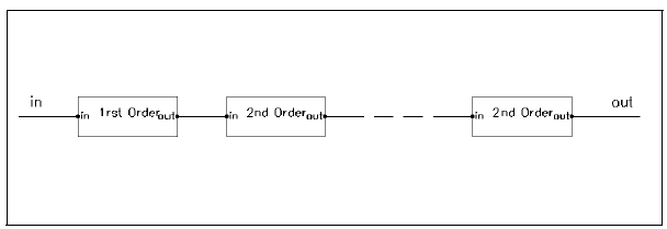
Figure 1: Square Roots Sub-circuit
The first- and second-order section transfer functions, H(s), are
H(s)=x/(s+x) ; x=2piαFc
H(s)=x2/(s2+(x/Q)s+x2); x=2piωFc
where s is the Laplace variable, and Fc is the filter cutoff frequency or bandwidth. The parameters α, ω, and Q define the pole positions of the various filtering responses.
Following is the behavioral Butterworth lowpass filter model text:
.SUBCKT butt_lp 1 2 params: Fc=1 ord=1 ;Subcircuit description
.PARAM pi=3.14159 ;Constant
.FUNC lp_1(x) {x/(s+x)} ;1st-order lowpass transfer function
*a1-a4 and b1-b4 determine which filter sections are selected, given the filter order
.PARAM a1={table(ord,1,1,2,0,3,1,4,0,5,1,6,0,7,1,8,0,9,1)}
.PARAM a2={stp(ord-1.5)}
.PARAM a3={stp(ord-3.5)} a4={stp(ord-5.5)} a5={stp(ord-7.5)}
.PARAM b1={1-a1} b2={1-a2} b3={1-a3} b4={1-a4} b5={1-a5}
*alpha, omega, and Q values of the Butterworth response for each section are looked up from these tables, based on the filter order. Upto 9th-order [ord] filter is allowed.
.PARAM alpha_b={table(ord,1,1,2,0,3,1,4,0,5,1,6,0,7,1,8,0,9,1)}
.PARAM omega1_b={table(ord,1,0,2,1,3,1,4,1,5,1,6,1,7,1,8,1,9,1)}
.PARAM Q1_b={table(ord,1,0,2,0.707,3,1,4,1.307,5,1.618,6,1.932,7,2.247,8,2.564,9,0.532)}
.PARAM omega2_b={table(ord,3,0,4,1,5,1,6,1,7,1,8,1,9,1)}
.PARAM Q2_b={table(ord,3,0,4,0.541,5,0.618,6,0.707,7,0.802,8,0.90,9,0.653)}
.PARAM omega3_b={table(ord,5,0,6,1,7,1,8,1,9,1)}
.PARAM Q3_b={table(ord,5,0,6,0.518,7,0.555,8,0.601,9,1)}
.PARAM omega4_b={table(ord,7,0,8,1,9,1)}
.PARAM Q4_b={table(ord,7,0,8,0.509,9,2.879)}
E 2 0 LAPLACE {V(1)}={(b1+a1*lp_1(2*pi*alpha_b*Fc))* ;VCVS with laplace description
+ (b2+a2*lp_2(2*pi*omega1_b*Fc,Q1_b))* ;1st order
+(b3+a3*lp_2(2*pi*omega2_b*Fc,Q2_b)) * ;2nd order
+(b4+a4*lp_2(2*pi*omega3_b*Fc,Q3_b)) *
+(b5+a5*lp_2(2*pi*omega4_b*Fc,Q4_b))}
.ENDs butt_lp ;end with subcircuit description
The model implements the overall voltage transfer function of the filter as shown in Figure 1 using a controlled voltage source (E component) that has the Laplace description. The model text shows that the model is limited to simulating a maximum of a ninth-order filter, which is made up of one first-order section and four second-order sections. It is often considered that a ninth-order filter is adequate for most applications. The filter model can easily be increased to simulate filters greater than 9th order by adding second-order sections. The transfer functions are specified through .FUNC statements. The parameters a1 through a4 and b1 through b4 determine which filter sections of the model are selected by using a simple selection algorithm, based on the order of the filter specified by the user. The selection algorithm is implemented using .PARAM statements as shown in the model text. The filter order is defined by the subcircuit parameter, ORD.
Note that the PSpice function stp, which is used in the model, describes a step function where stp(x) is 1 if x>0 and is 0 otherwise. The α, ω, and Q values of the Butterworth response are defined as lookup tables using .PARAM statements. These values are looked up automatically given the order of the filter. The model is described as a sub-circuit called Butt_LP with the input at node in and the output at node out as shown in Figure 2.
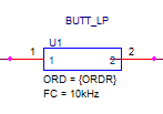
Figure 2: Lowpass Filter Circuit
The sub-circuit has two parameters: the filter cutoff frequency (FC) and its order (ORD). These subcircuit parameters are given default values, which are arbitrarily set to 1. They will be changed to the required cutoff frequency and order when the subcircuit is called.
To illustrate the use of the models, consider the following example. Here, the Butterworth lowpass filter model is used to obtain a family of curves for second- through ninth-order responses. Assume the filter has a cutoff frequency of 10 kHz. Using Capture, the following circuit is drawn.
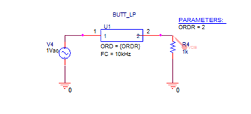
Figure 3: Butterworth lowpass filter model
The filter Butt_LP has an AC source on its input and a 1K load resistor on its output. On the Butt_LP symbol, the attribute FC has a value of 10K, and ORD is set to the global variable defined in the global parameter block (PARAM). Finally, a VDB voltage marker is placed on the output node to view the results.
The PSpice simulation consists of a 1000-point linear AC sweep and a parametric analysis. The parametric analysis steps the global parameter, ORD, from 2 to 9. The simulated frequency response of the filter for various orders is shown in Figure 4.

Figure 4: frequency Response of the Butterworth lowpass filter model
Butt_HP (Butterworth filter)Three highpass filter models are developed similar to the lowpass filter models. The three models are:
Each model is capable of simulating up to a ninth-order filter and is used in a similar manner to that of the lowpass as described in Example 1
To illustrate the use of the models, consider the following example. Here, the Butterworth highpass filter model is used to obtain a family of curves for second- through ninth-order responses. Assume the filter has a cutoff frequency of 1 kHz. Using Capture, the following circuit is drawn:
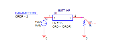
Figure 5: Butterworth highpass filter model
The filter Butt_HP has an AC source on its input and a 1K load resistor on its output. On the Butt_HP symbol, the attribute FC has a value of 1K, and ORD is set to the global variable defined in the global parameter block (PARAM). Finally, a VDB voltage marker is placed on the output node to view the results.
The PSpice simulation consists of a 1001-decade logarithmic AC sweep and a parametric analysis. The parametric analysis steps the global parameter, ORD, from 2 to 9. The simulated frequency response of the filter for various orders is shown in Figure 6.
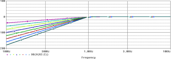
Figure 6: Frequency response of the Butterworth highpass filter model for various orders
The three bandpass filter models are:
One approach to obtain bandpass filters is to cascade lowpass and highpass circuits. The cutoff frequency of the lowpass circuit defines the lower -3 dB point of the bandpass filter bandwidth, while the cutoff frequency of the highpass filter defines the upper -3 dB point of the filter bandwidth. On the basis of this approach and by using the lowpass and highpass filter models discussed earlier, a behavioral bandpass filter model can be defined and that is shown in Figure 7.
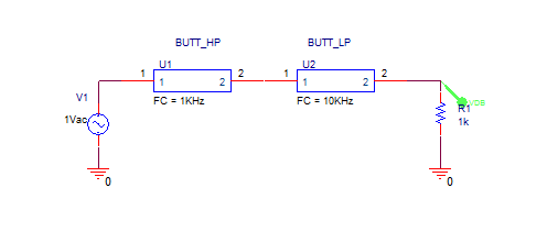
Figure 7: Butterworth bandpass filter model
Now you will simulate the bandpass circuit that has the following specifications: Lower-3dB = 1 kHz, Upper-3dB = 10 kHz, 30dB minimum at 0.2 kHz and 50 kHz.

Figure 8: Frequency response of the Butterworth bandpass filter model
The Butt_HP filter symbol has a attribute FC = 1kHz and the Butt_HP filter symbol has a attribute FCH = 5kHz for low and high cutoff frequencies, respectively. A single AC source is frequency swept over 0.2 kHz to 50 kHz (1001 decade). The simulated frequency response of the filter is shown in Figure 8.
Butt_BR (Butterworth filter)The Band-Reject Filter model is based on summing outputs of the lowpass and highpass filter models. The cutoff frequency of the lowpass circuit defines the lower -3dB point of the bandpass filter bandwidth, while the cutoff frequency of the highpass circuit defines the upper -3dB point of the filter bandwidth.
The three band-reject filter models are:
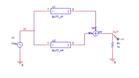
Figure 9: Band Reject filter Circuit
Figure 10 shows the simulation response of the Band Reject Filter circuit.
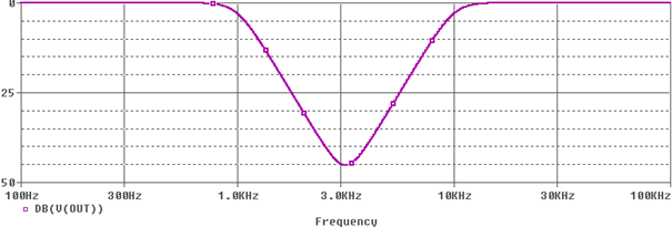
Figure 10: Frequency Response of the Band Reject Filter Circuit
Figure 11 shows a fifth-order, 0.25dB ripple Chebyshev bandreject filter with a lower -3dB point at 100 Hz and the upper -3dB point at 1 kHz.
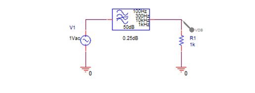
Figure 11: Chebyshev band-reject filter circuit
In Figure 12, you can see that the frequency response of the Chebyshev band-reject filter circuit. Notice that the frequency response of a general band-reject filter circuit is different than the one by a Chebyshev band-reject filter circuit.
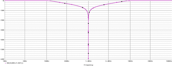
Figure 12: Frequency response of the Chebyshev band-reject filter circuit
© Copyright 2016 Cadence Design Systems, Inc. All rights reserved. Cadence, the Cadence logo, and Spectre are registered trademarks of Cadence Design Systems, Inc. All others are properties of their respective holders.
Copyright © 2024 Cadence Design Systems, Inc. All rights reserved.
